Code examples

Note

More examples will be provided on request.

Plot time series and power spectral density

Import the time series database, load data from file and plot all time series.

"""
Example of using the time series database class
"""
import os

from qats import TsDB

db = TsDB()

# locate time series file
file_name = os.path.join("..", "..", "..", "data", "mooring.ts")

# load time series from file
db.load([file_name])

# plot everything on the file

You can also select a subset of the timeseries (suports wildcards) as shown below.

# plot only specific time series identified by name

You can also plot the power spectral density of the selected time series. Because the ‘surge’ time series was sampled at a varying time step the the time series are resampled to a constant time step of 0.1 seconds before the FFT.

# plot the power spectral density for the same time series

Count cycles using the Rainflow algorithm

Note

Some of the syntax shown below is not applicable for version <= 4.6.1, in particular the unpacking of cycles. The changes implemented since 4.6.1 are backwards compatible, however; the syntax suggested below is recommended due to better performance. One may also experience minor changes in rebinned cycles. Finally, the mesh established by qats.fatigue.rainflow.mesh() (and used by TimeSeries.plot_cycle_rangemean3d()) was not correct for version <= 4.6.1. For more details, please refer to the CHANGELOG.

Fetch a single time series from the time series database, extract and visualize the cycle distribution using the Rainflow algorithm.

"""
Example on working with cycle range and range-mean distributions.
"""
import os

from qats import TsDB

# locate time series file
file_name = os.path.join("..", "..", "..", "data", "simo_p_out.ts")

# load time series directly on db initiation
db = TsDB.fromfile(file_name)

# fetch one of the time series from the db
ts = db.get(name='tension_2_qs')

# plot its cycle ranges as bar diagram
ts.plot_cycle_range(n=100)

# plot its cycle-range-mean distribution as scatter
ts.plot_cycle_rangemean(n=100)

# ... or as a 3D surface.
ts.plot_cycle_rangemean3d(nr=25, nm=25)

# you can also collect the cycle range-mean and count numbers (see TimeSeries.rfc() and TimeSeries.get() for options)
cycles = ts.rfc()

# unpack cycles to separate 1D arrays if you prefer

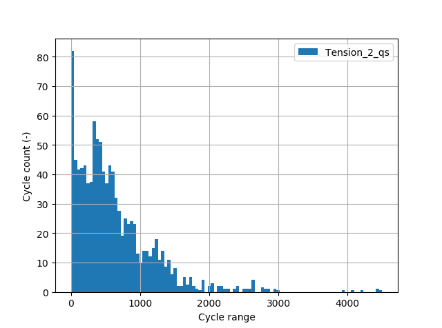
Single cycle range distribution.

Single cycle range-mean distribution.

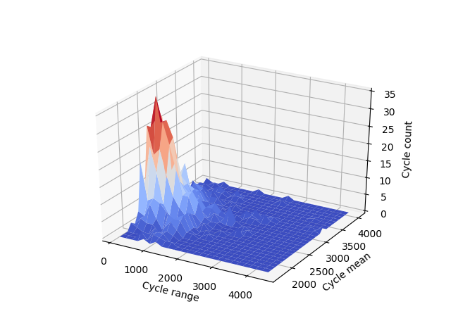
Single 3D cycle range-mean distribution

Compare the cycle range and range-mean distribution from several time series using the methods on the TsDB class.

ranges, means, counts = cycles.T

# The TsDB class also has similar methods to ease comparison
# compare cycle range distribution (range versus count) grouped in 100 bins
db.plot_cycle_range(names='tension*', n=100)

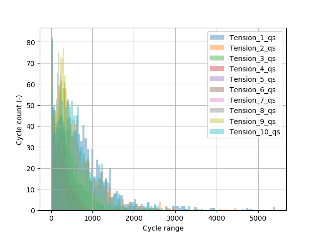
Comparison of several cycle range distributions.

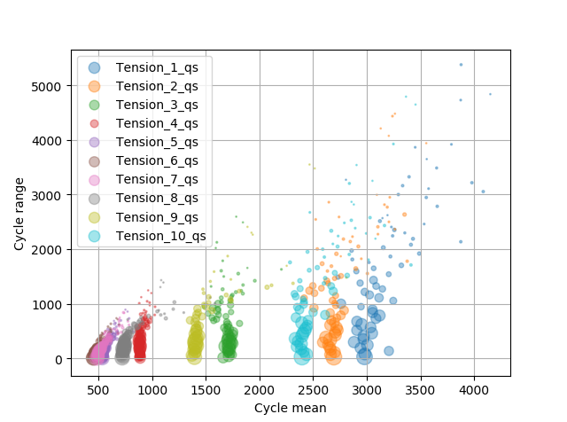
Comparison of several cycle range-mean distributions.

Calculate fatigue damage in mooring lines

Using a traditional S-N curve with constant slope and intercept.

"""
Calculate mooring line fatigue.
"""
import os
from math import pi

import numpy as np

from qats import TsDB
from qats.fatigue.sn import SNCurve, minersum

# load time series
db = TsDB.fromfile(os.path.join("..", "..", "..", "data", "simo_p_out.ts"))

# initiate SN-curve: DNVGL-OS-E301 curve for studless chain
sncurve = SNCurve(name="Studless chain OS-E301", m1=3.0, a1=6e10)

# Calculate fatigue damage for all mooring line tension time series (kN)
for ts in db.getl(names='tension_*_qs'):
    # count tension (discarding the 100s transient)
    cycles = ts.rfc(twin=(100., 1e12))

    # unpack cycle range and count as separate lists (discard cycle means)
    ranges, _, counts = cycles.T

    # calculate cross section stress cycles (shown here: 118mm studless chain, with unit [kN] for tension cycles)
    area = 2. * pi * (118. / 2.) ** 2.          # mm^2
    ranges = [r * 1e3 / area for r in ranges]   # MPa

    # calculate fatigue damage from Palmgren-Miner rule (SCF=1, no thickness correction)
    damage = minersum(ranges, counts, sncurve)

    # print summary
    print(f"{ts.name}:")
    print(f"\t- Max stress range = {max(ranges):12.5g} MPa")
    print(f"\t- Total number of stress ranges = {sum(counts)}")
    print(f"\t- Fatigue damage = {damage:12.5g}\n")

Apply low-pass and high-pass filters to time series

Initiate time series database and load time series file in one go. Plot the low-passed and high-passed time series and the sum of those.

"""
Example showing how to directly initiate the database with time series from file and then filter the time series.
"""
import os

import matplotlib.pyplot as plt

from qats import TsDB

# locate time series file
file_name = os.path.join("..", "..", "..", "data", "mooring.ts")
db = TsDB.fromfile(file_name)
ts = db.get(name="Surge")

# Low-pass and high-pass filter the time series at 0.03Hz
# Note that the transient 1000 first seconds are skipped
t, xlo = ts.get(twin=(1000, 1e12), filterargs=("lp", 0.03))
_, xhi = ts.get(twin=(1000, 1e12), filterargs=("hp", 0.03))

# plot for visual inspection
plt.figure()
plt.plot(ts.t, ts.x, "r", label="Original")
plt.plot(t, xlo, label="LP")
plt.plot(t, xhi, label="HP")
plt.plot(t, xlo + xhi, "k--", label="LP + HP")
plt.legend()
plt.grid(True)
plt.show()

Tail fitting with Weibull

Fit a parametric Weibull distribution to the largest 13% of the peak sample. Often called tail fitting.

"""
Example showing tail fitting with Weibull
"""
import os

from qats import TsDB
from qats.stats.weibull import lse, plot_fit

# locate time series file
file_name = os.path.join("..", "..", "..", "data", "mooring.ts")
db = TsDB.fromfile(file_name)
ts = db.get(name="mooring line 4")

# fetch peak sample
x = ts.maxima()

# fit distribution to the values exceeding the 0.87-quantile of the empirical cumulative distribution function
a, b, c = lse(x, threshold=0.87)

# plot sample and fitted distribution on Weibull scales
plot_fit(x, (a, b, c))

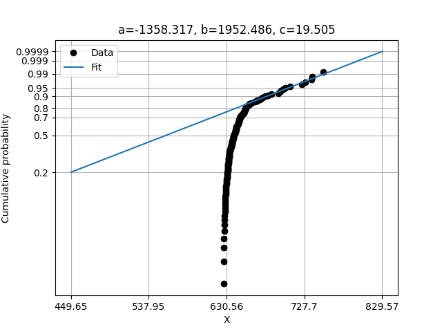
Comparison of empirical sample distribution and fitted parametric distribution on linearized scales.

Merge files and export to different format

Todo

Coming soon